Irregular Tributary Areas and How To Best Calculate Them

This article presents a method for calculating tributary areas of columns in irregular grid layouts with 7 simple steps.

Tributary Areas

Tributary area is a concept used by engineers to estimate design loads of structural elements subjected to vertical surface loading. The basic idea is to geometrically derive an approximation of how much area each column, wall or beam has to carry given a specific configuration. The load is typically dead load or live load applied at the surface.

We have previously covered the basics of calculating tributary areas of regular layouts in the article Tributary areas of columns and how to best calculate them. However, it becomes slightly trickier to derive estimations of the tributary area when the column layout is irregular. But don’t fret – there is a simple method in 7 steps to tackle this challenge, which will be presented shortly in this article.

Irregular Column Layouts

The article mentioned above presents a method for calculating tributary areas using an example structure with its columns organized in an orthogonal grid. This is typically referred to as a “regular layout“, or a layout with evenly spaced gridlines. That means that the column tributary areas can easily be calculated by measuring half the distance between the gridlines as described in detail in the article.

However, not all structures have their columns organized in a regular grid. Depending on the architectural design intent, the gridlines can be much more complex and irregular (See figure below for example). For this scenario, we need more flexible approach for calculating the tributary area.

The General Approach

The general approach for calculating irregular tributary areas is inspired by Voronoi diagrams. As opposed to relying on regular gridlines, it uses the geometric topology of the configuration to derive the centerline panel of each column.

Here are the 7 steps that summarize the procedure:

• Select a column in the configuration
• Identify its closest neighboring columns
• Draw connectivity lines between the column and its neighbors
• Identify the mid points of the connectivity lines
• Starting from the mid points, draw perpendicular lines in each direction
• Let the perpendicular lines instersect and form a polygon
• Calculate the area of the polygon

The area of the resulting polygon will be the tributary area of the column. We can repeate this process for every column in the configuration.

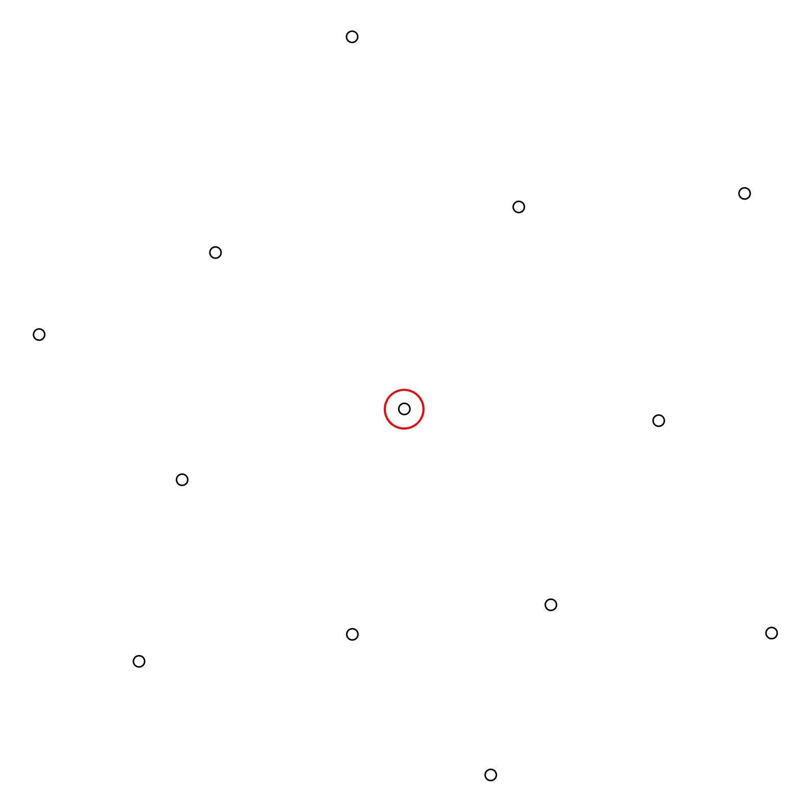
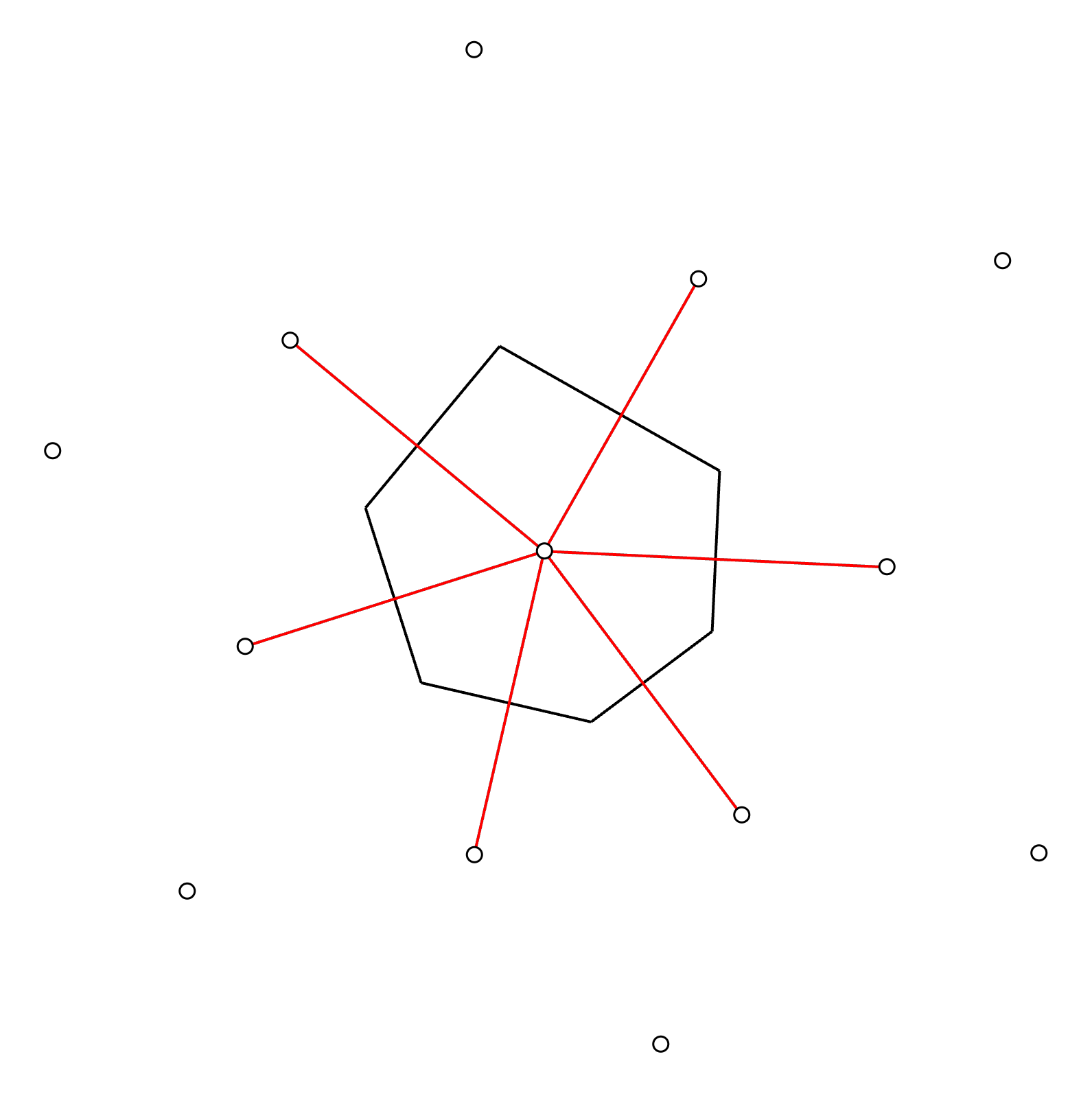
Simple, eh? Let’s go through these steps using the irregular configuration below as an example. Each dot represents a column in plan:

Step 1: Select a column

The first step is to select an arbitrary column in the configuration to start the procedure with. It can be convenient to start with an interior column, because they usually have a higher number of neighbors. Here we select the column highlighted with a red circle:

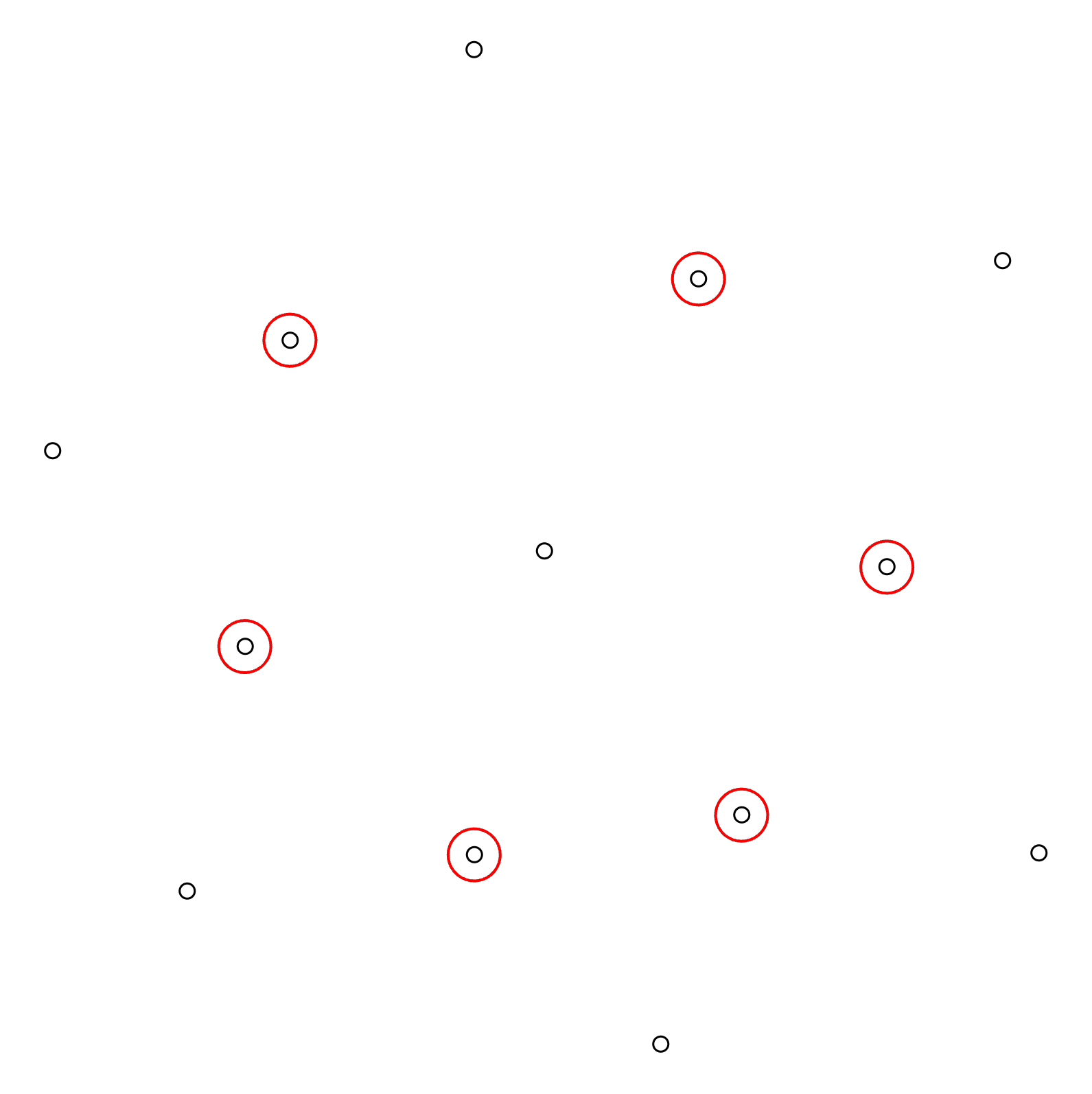
Step 2: Identify Closest Neighbors

With one column selected, the next step is to identify its closest neighboring columns in all directions. For the selected column in this demonstration, the highlighted dots have been identified as neighboring columns:

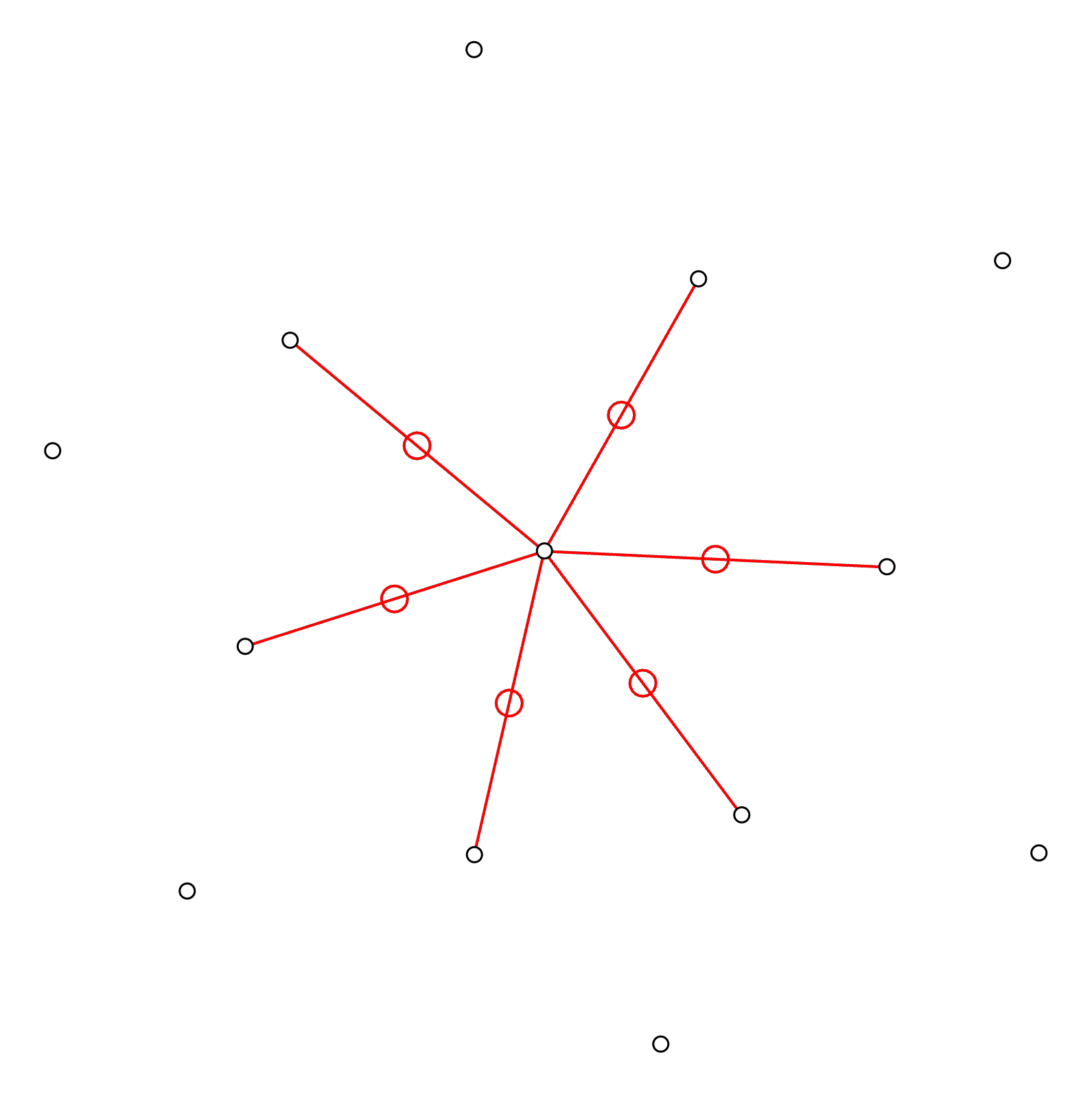
Step 3: Draw connectivity lines

When we have identified the neighboring columns, we can proceed with drawing connectivity lines between those and the selected column.

Step 4: Identify mid points

The next step is to identify the mid points on each connectivity line. We can do this by simply measuring the distance of each line and divide it by two.

Step 5: Draw perpendicular lines

Starting from the mid points on each connectivity line, we shall now draw perpendicular lines in each direction. Extend the lines until they intersect.

Step 6: Form polygon

With the extended perpendicular lines, we can see that a polygon is emerging with its vertices generated by the intersection points.

Step 7: Calculate the area of the polygon

The area of the resulting polygon will be the tributary area of the column! In this case, the resulting polygon is irregular .The area of an irregular polygon can be calculated in many different ways. The most popular methods are based on the concept to divide the polygon into smaller regular polygons (triangles for instance). For example, see this article for more details on this. If you are using CAD software (for instance AutoCAD), then there is usually an area command or tool that can be used.

That’s it! It isn’t harder than this. Now let’s take a look at an example.

Example of Calculating Irregular Tributary Areas

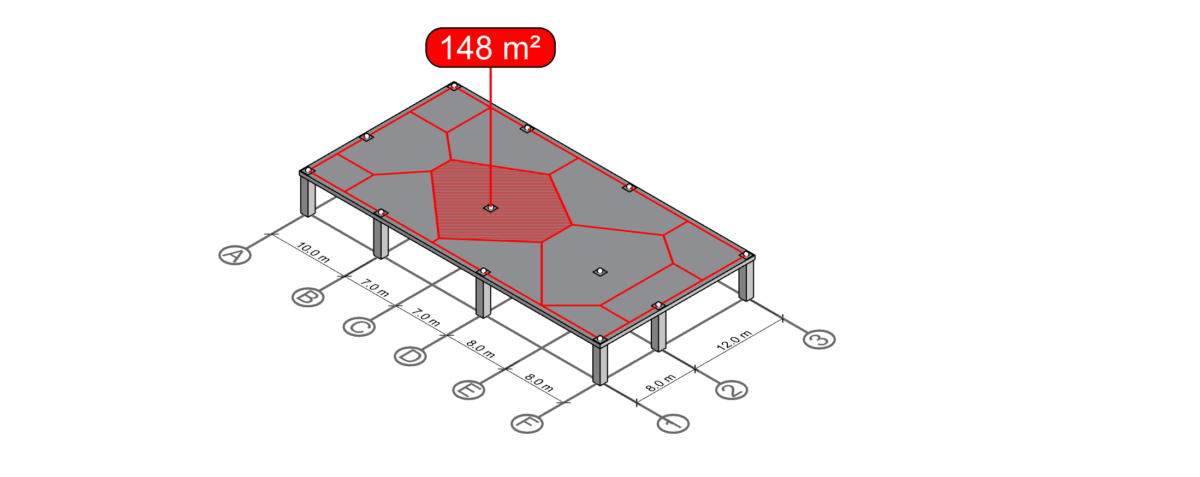
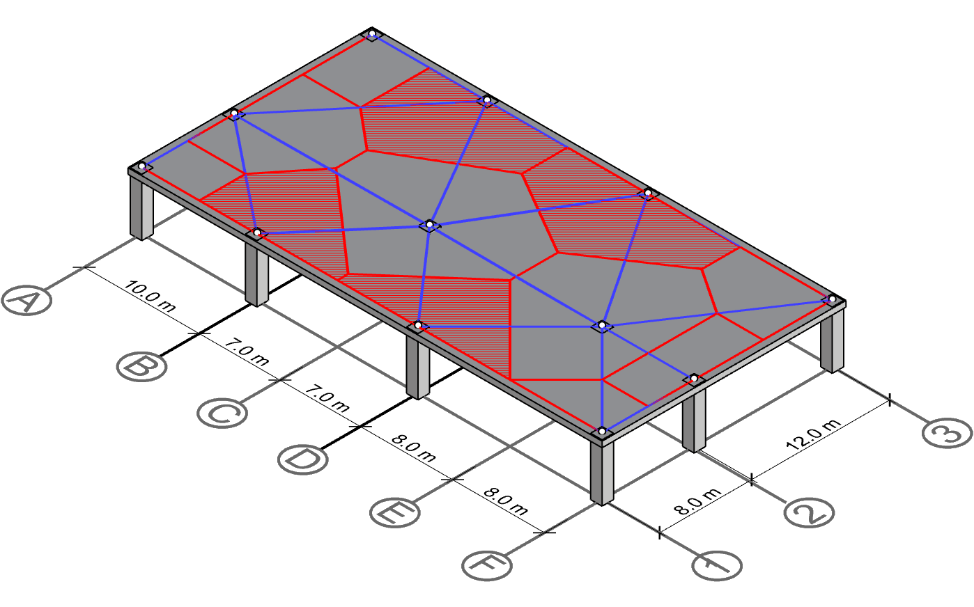
Let’s take a look at a more realistic scenario and follow the presented steps to demonstrate how the procedure above can be applied to buildings.

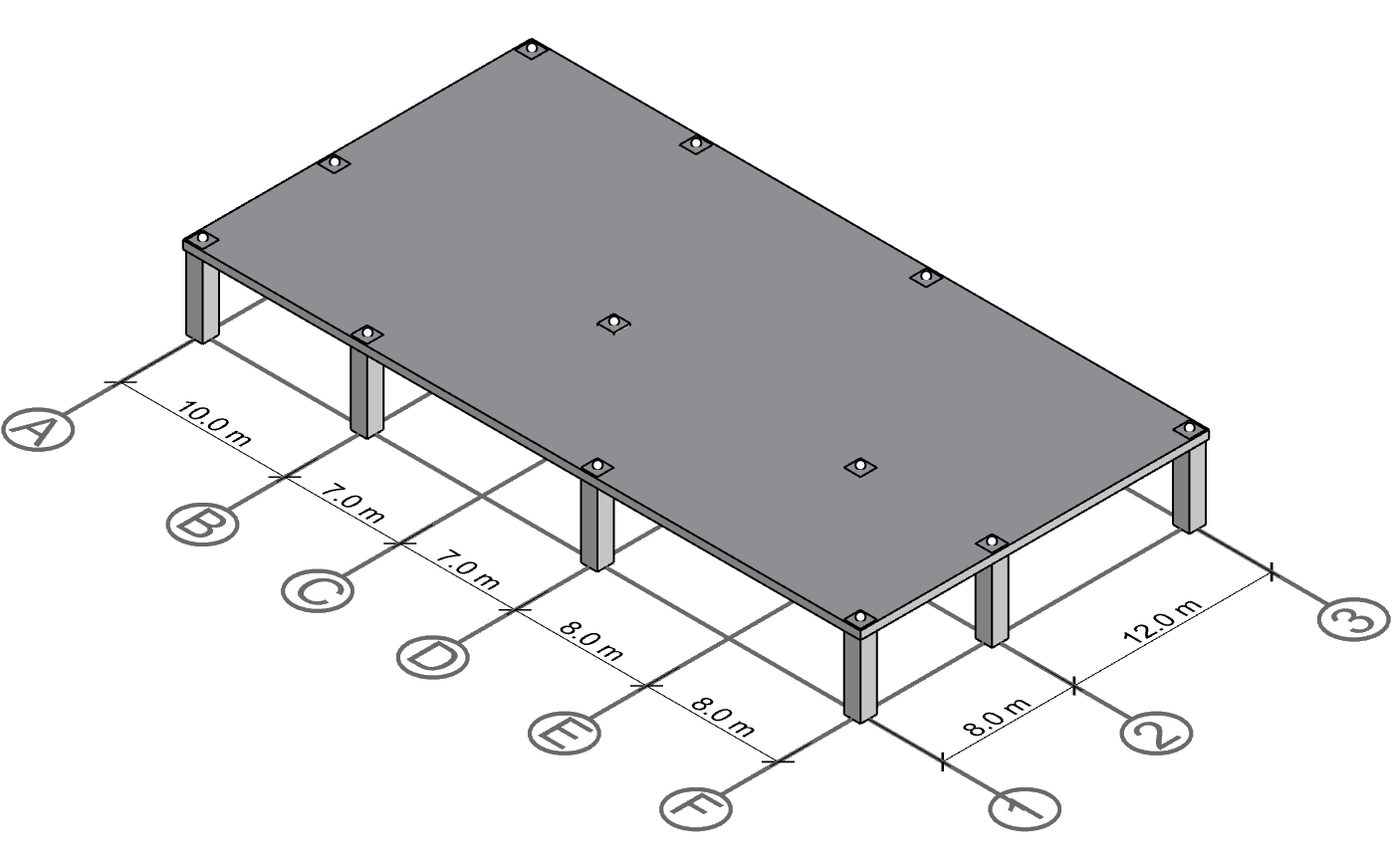
The structure has 6 gridlines in one direction (A-F) and 3 gridlines in the other direction (1-3). The two gridline directions are orthogonal, but there isn’t a column on every intersection. For instance, gridline intersection E-1, E-3, C-1 and C-3 do not have columns.

Let’s run through the steps and see what that gives us.

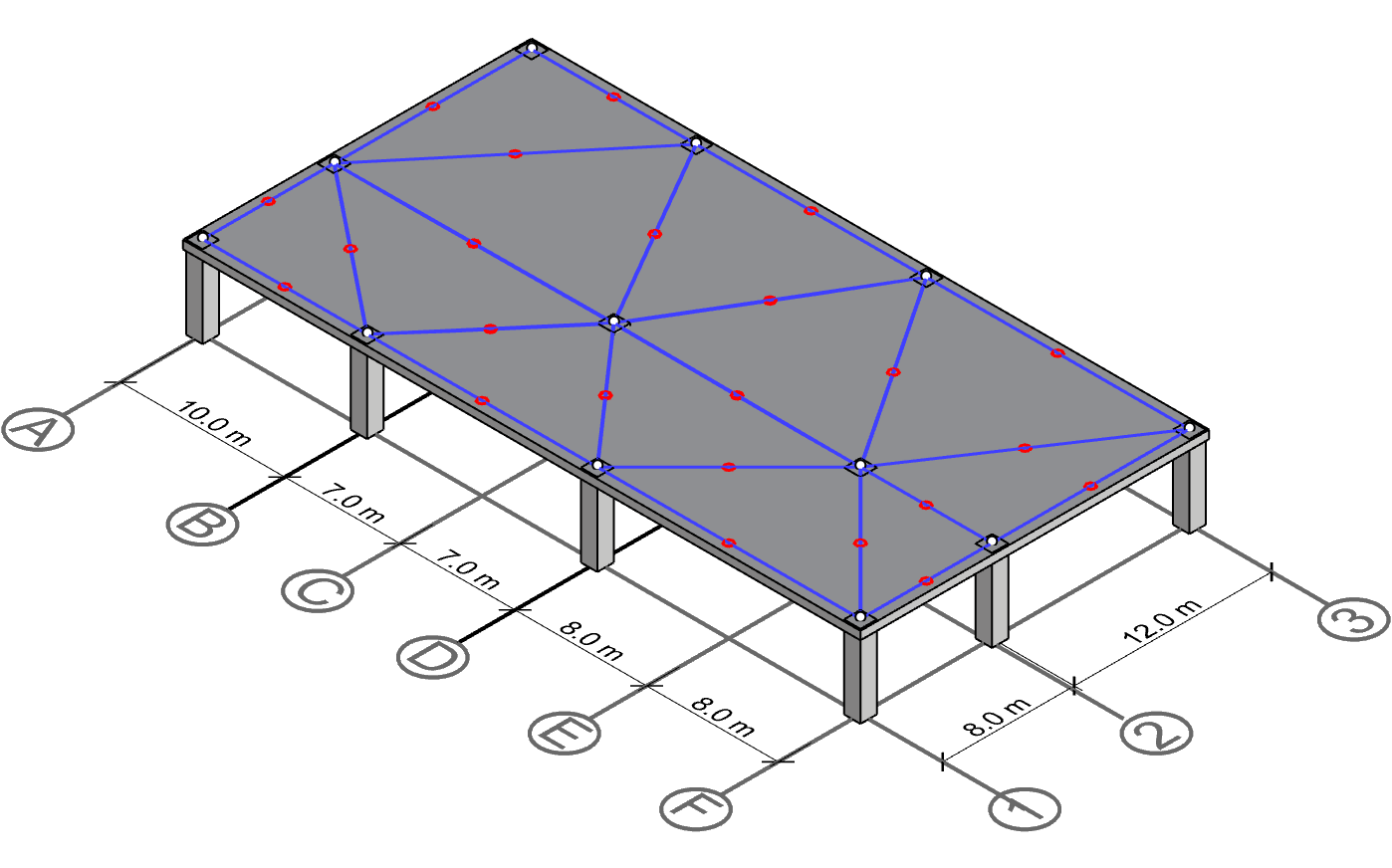
Draw connectivity lines

The first step is to draw the connectivity lines between the columns. In the image below, we have drawn connectivity lines for all columns (as opposed to starting with one). Note that the connectivity lines should always form a triangular pattern. This is also known as Delaunay triangulation.

Identify mid points

Identifying the mid points on the connectivity lines is straight forward as mentioned. Just measure the distance of each line and divide by 2.

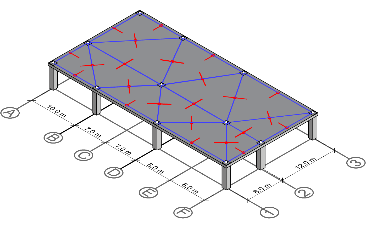
Drawing perpendicular lines from the mid points

Each mid point now gets a pair of lines perpendicular to the connectivity lines. Note that we can only extend some lines in one direction:

• If the mid point is on a line that is shared by two triangles, then two perpendicular lines are drawn in each direction.
• If the mid point is on a line that is shared by only one triangle, then one perpendicular line is drawn (happens at the perimeter).

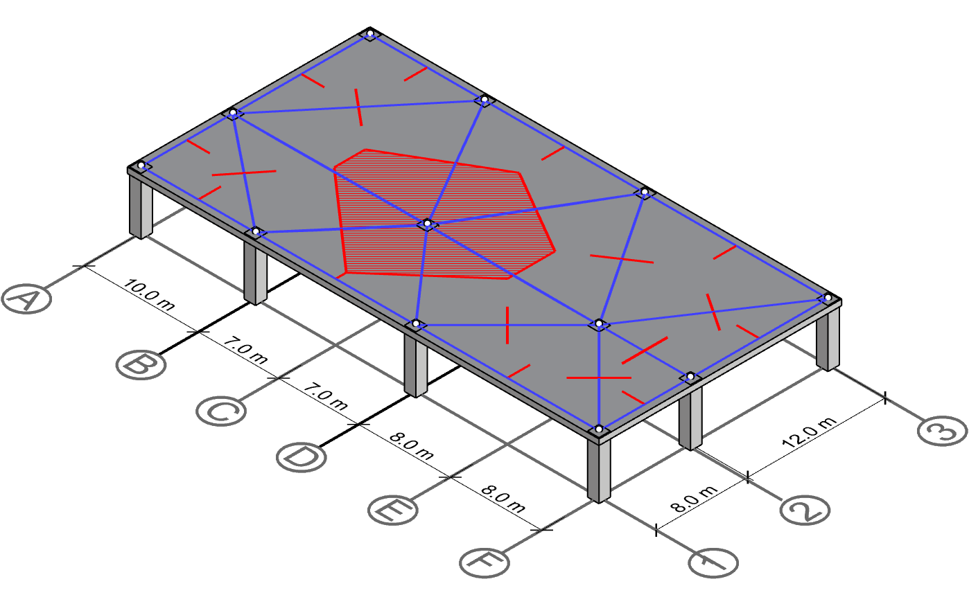
Polygon for column C-2

Starting with column C-2, we can form the centerline polygon by intersecting the perpendicular lines surrounding the column.

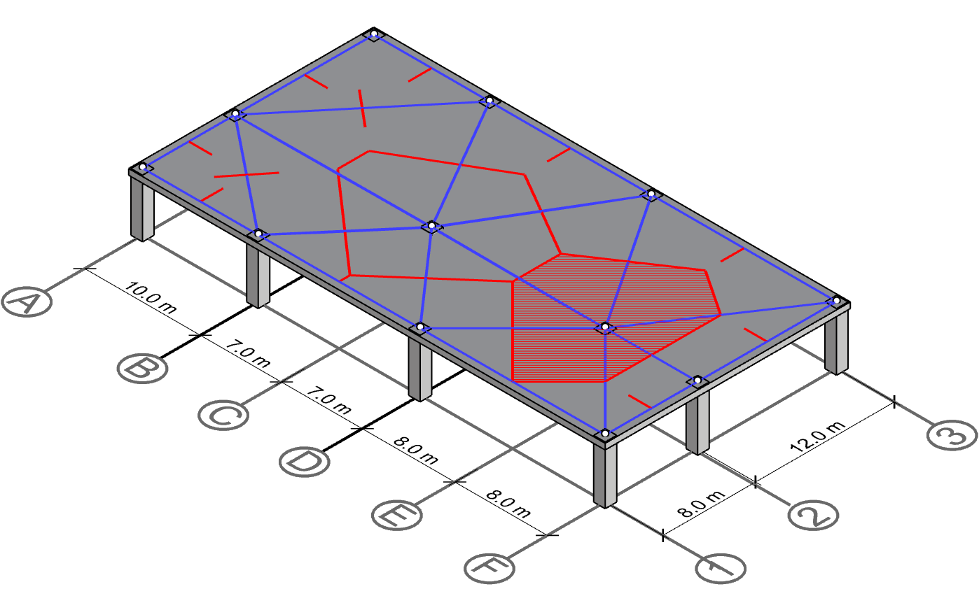
Polygon for column E-2

Running the same procedure on column E-2 gives us a similar hexagon. Note that the two polygons share a common edge.

Polygon for column A-2 and F-2

With C-2 and E-2 calculated, we can proceed with the last two columns on gridline 2. Since both of these columns are exterior columns, they have fewer neighbors and therfore smaller tributary area than interior columns.

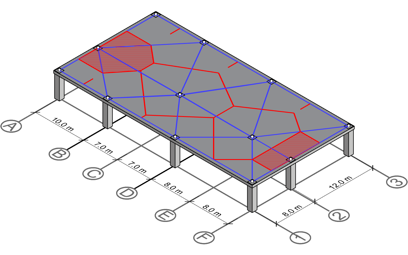
Polygon for column A-1, A-3, F-1 and F-3

Even fewer neighbors do the corner columns have at A-1, A-3, F-1 and F-3 have. Therefore, the polygons for those become relatively simple to draw.

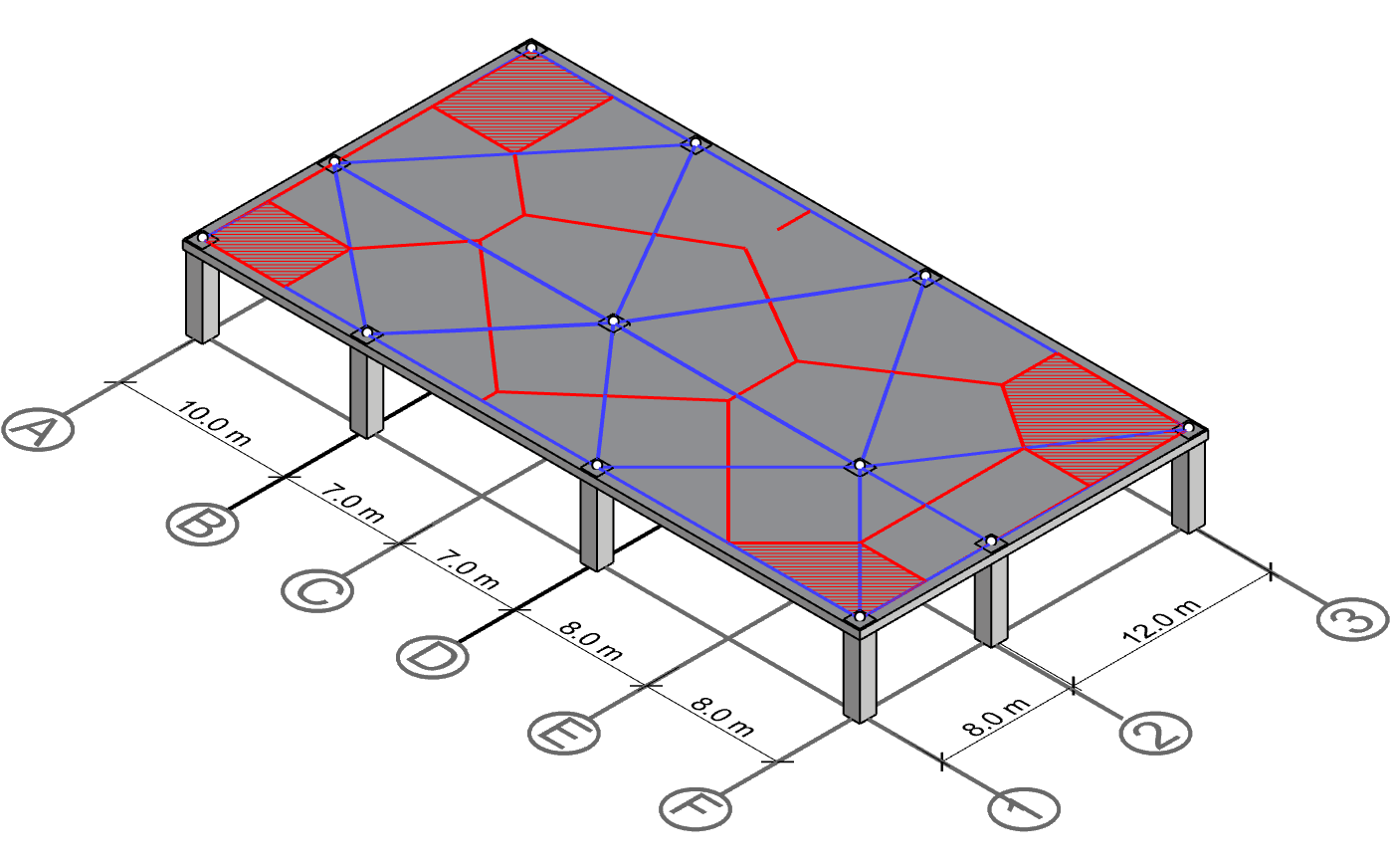
Polygon for column B-1, B-3, D-1 and D-3

Finally yet importantly, the polygons for columns along gridline B and C shall be drawn. Note that we have already drawn most of the perpendicular lines and used them for neighboring columns.

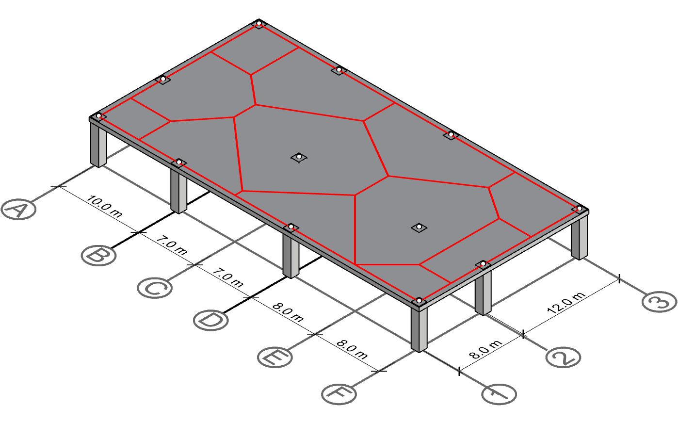
Calculate polygon areas

At this stage, we have derived the centerline panels for all columns, and hence arrived at the final solution. As previously described, these polygons make up the visual representation of the tributary areas of each column they enclose. The only step left to do is to calculate the areas of these polygons. For more information on how to do that, please see step 7 in the previous chapter.

Conclusion

In this article we have presented a general method for calculating tributary areas of columns in irregular layouts. When combined with structural pressures from the dead load and/or live load, we can easily calculate column forces to use for further structural design.

You can execute the 7 step process described in the article using pen and paper or CAD software. However, for larger configurations potentially involving hundreds of columns, this can get very time consuming and tedious. There we recommend you to automate the process with structural analysis software.

A software that can efficiently calculate column tributary areas of irregular configurations is Tribby3d. It is a cloud based and easy-to-use structural analysis software with excellent capabilities to visualize and compute tributary areas of both columns and walls. See below for a demo of running through the example presented above using the software.

If you’re interested in testing the free beta version of Tribby3d and calculate irregular tributary areas, please sign up here: https://tribby3d.com/sign-up

You can also test an open version of Tribby3d here, without the requirement to sign-up: Free Tributary Area Calculator.

Related Articles